Delete Blank Rows in Ms Excel: Step-by-step Guide

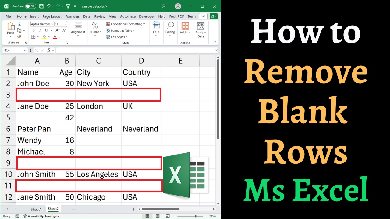
Tired of those pesky blank rows messing up your Excel spreadsheets? Whether you’re dealing with data imports, user errors, or just plain messy files, blank rows can be a real headache. They disrupt sorting, filtering, and formulas, making your data analysis a nightmare.

This guide will equip you with the ultimate arsenal of techniques to obliterate blank rows and restore order to your Excel kingdom. We’ll explore various methods, from simple clicks to powerful shortcuts, ensuring you have the perfect solution for any situation.

Method 1: The “Go To Special” Blitz

This classic technique is a quick and efficient way to eliminate blank rows. Here’s how to unleash its power:

1. Select Your Battlefield: Highlight the entire range of data containing those pesky blank rows.
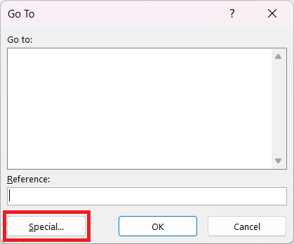
2. Launch the “Go To Special” Command: Press F5 (or Ctrl+G) to open the “Go To” dialog box. Then, click “Special…”.
   
3. Target the Enemy: In the “Go To Special” dialog box, select “Blanks” and click “OK”. This will highlight all the empty cells within your selection.
   
4. Execute the Deletion: With the blank cells selected, press Ctrl+-(minus sign). Excel will prompt you to confirm the deletion of entire rows. Click “OK” to banish those blank rows forever.
   

Method 2: The “Filter and Destroy” Tactic

For those who prefer a more visual approach, the filter method offers a precise way to identify and eliminate blank rows. Here’s how to deploy this tactic:

1. Activate the Filter: Select the header row of your data and click on the “Filter” button in the “Data” tab (or press Ctrl+Shift+L).
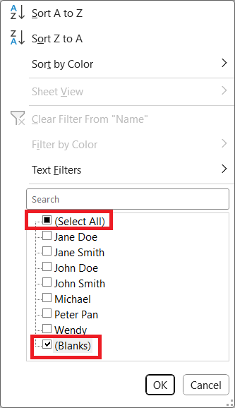
2. Isolate the Empty Rows: Click on the filter dropdown arrow in the column where blank rows are most obvious. Uncheck “Select All” and then check the box next to “(Blanks)”. This will filter out all rows except those with blank cells in the selected column.
   
3. Annihilate the Blanks: Select the filtered blank rows by clicking on the row numbers. Right-click on the selection and choose “Delete Row” (or press Ctrl+-(minus sign)).
   
4. Deactivate the Filter: Once the blank rows are gone, click the “Filter” button again to display all your data.

Method 3: The “Sort and Conquer” Strategy

If you need to preserve the order of your data while removing blank rows, sorting is your secret weapon. Follow these steps:

1. Add a Helper Column: Insert a new column next to your data. In the first cell of this column, enter the number 1.
2. Number the Rows: Fill the rest of the helper column with sequential numbers (2, 3, 4, etc.). You can use the fill handle to quickly drag the numbers down.
3. Sort by a Relevant Column: Choose a column with data that will effectively push the blank rows to the bottom when sorted. Click on the “Sort & Filter” button in the “Data” tab and select the appropriate sorting order.
4. Eliminate the Empty Rows: Scroll to the bottom of your data where the blank rows have congregated. Select these rows and delete them using the methods described earlier.
5. Restore the Original Order: Sort your data again using the helper column to return your data to its original sequence.
6. Remove the Helper Column: Once you’re satisfied, delete the helper column.

Method 4: The “COUNTA” Code of Silence

For the Excel ninjas who love formulas, the COUNTA function offers a powerful way to identify and eliminate blank rows. Here’s the secret code:

1. Insert a “Blank Detector” Column: Add a new column to your spreadsheet.
2. Apply the COUNTA Formula: In the first cell of this column, enter the following formula: =COUNTA(A1:Z1) (replace “A1:Z1” with the actual range of cells in the first row of your data). This formula counts the number of non-blank cells in the row.
3. Extend the Formula: Drag the fill handle down to apply the formula to all rows in your data.
4. Filter for Zero Counts: Apply a filter to the “Blank Detector” column and select only the rows with a count of zero. These are your completely blank rows.
5. Delete and Conquer: Delete the filtered blank rows and remove the filter to reveal your clean data.

Frequently Asked Questions

• Q: What if I only want to remove rows with blank cells in specific columns?
  • A: You can adapt the “Filter and Destroy” method by filtering multiple columns simultaneously. Select the desired columns, apply the filter, and choose “(Blanks)” for each column. This will isolate rows with blank cells in all specified columns.
• Q: Can I prevent blank rows from appearing in the first place?
  • A: Yes! When importing data, use the “Remove Duplicates” feature to eliminate duplicate blank rows. You can also use data validation to prevent users from entering blank rows in specific columns.
• Q: How do I remove blank rows in a large dataset with thousands of rows?
  • A: The “Go To Special” and “Filter and Destroy” methods are generally efficient even for large datasets. However, for extremely large datasets, consider using VBA macros to automate the process.

Related Posts

• Automated interpolation formula for Excel: Define excel interpolate function & use it forever
• Evaluates String as if it Were a Formula in Excel
• How to Remove Duplicate Values in MS Excel
• How to check if excel cell is empty or blank
• How to enable fill handle/formula drag-and-drop handle in Ms Excel
• How to make a macro available in all workbooks
• How to sort columns in Excel
• Tutorial on how to Add a Dropdown List in Excel

C P Gupta

C P Gupta is a YouTuber and Blogger. He is expert in Microsoft Word, Excel and PowerPoint. His YouTube channel @pickupbrain is very popular and has crossed 9.9 Million Views.